Alternative titles: Applying the Feynman Technique to Understanding the
Transformer Architecture, or The Life of a Token Inside a Transformer,
or The Transformer for the Impatient.
In 2017, researchers at Google publish the
Attention Is All You Need paper, in which they introduce
the Transformer architecture. The world runs with it.
Soon after, researchers at OpenAI develop a belief that this architecture scales
better than anything they’ve seen. In 2020, they publish the
Scaling Laws for Neural Language Models paper and keep feeding
data and compute to a variant of the Transformer, which they then teach to
follow instructions. In November 2022, ChatGPT is born.
The field has moved fast since, but today’s large language models (LLMs)
are still Transformers. Understanding the original gives you a point of
reference for everything that came after. At least that’s my bet.
So let’s travel back to 2017 and figure out how the sausage token is made.
My focus here is on the arithmetic, not intelligence.
High-level Overview
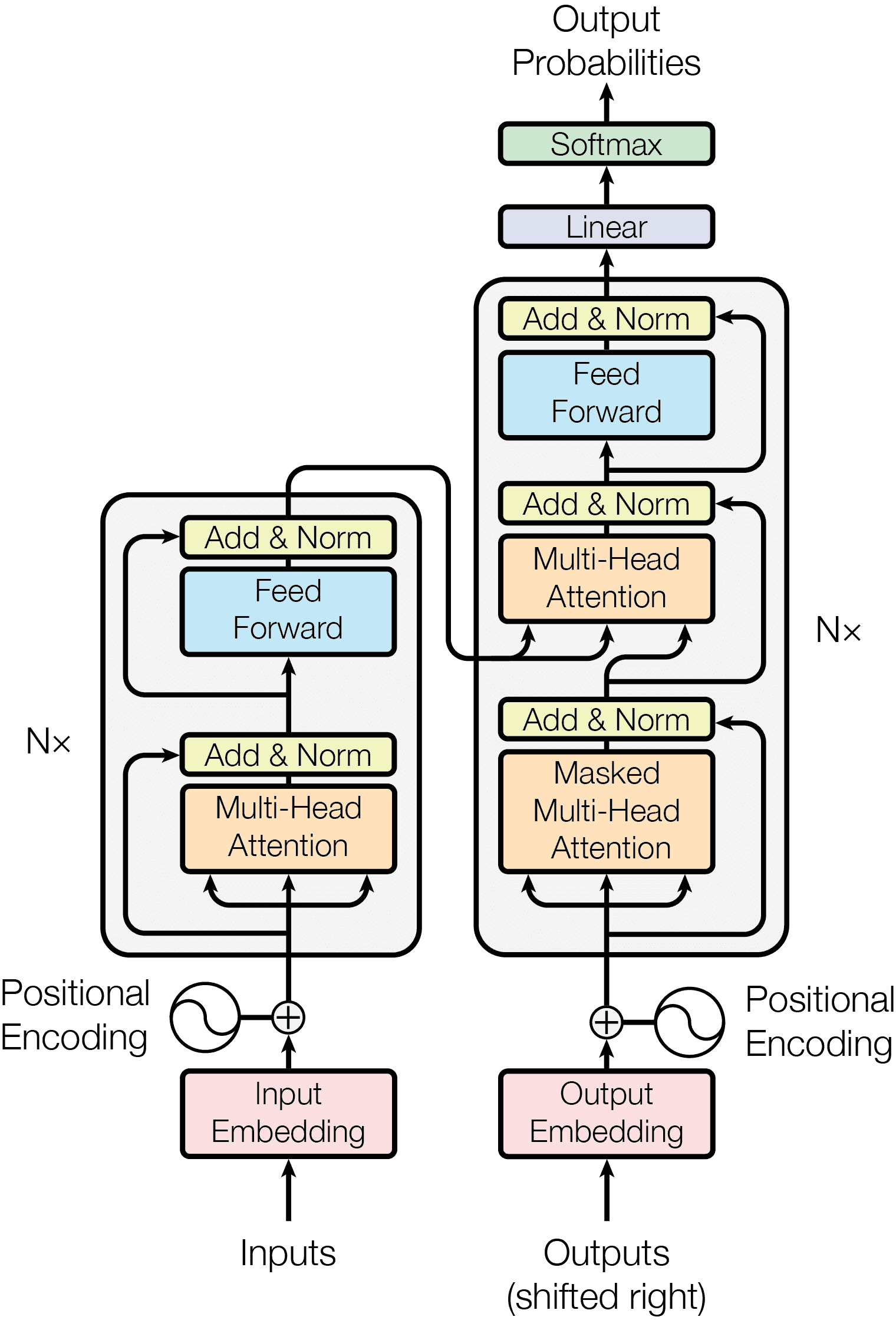
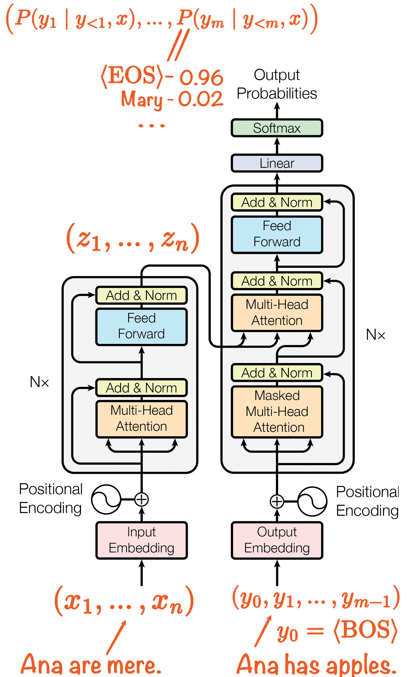
The Transformer - model architecture. Figure 1 from Attention Is All You Need (Vaswani et al., 2017).
The Transformer is introduced as a transduction model, mainly in the context
of machine translation. That is, the model takes a phrase in one language
and transforms (transduces) it into another.
Let’s pick an example we’ll follow through the rest of the note:
RomanianAna are mere.p⟶EnglishAna has apples.
The Model Architecture section of the paper opens with:
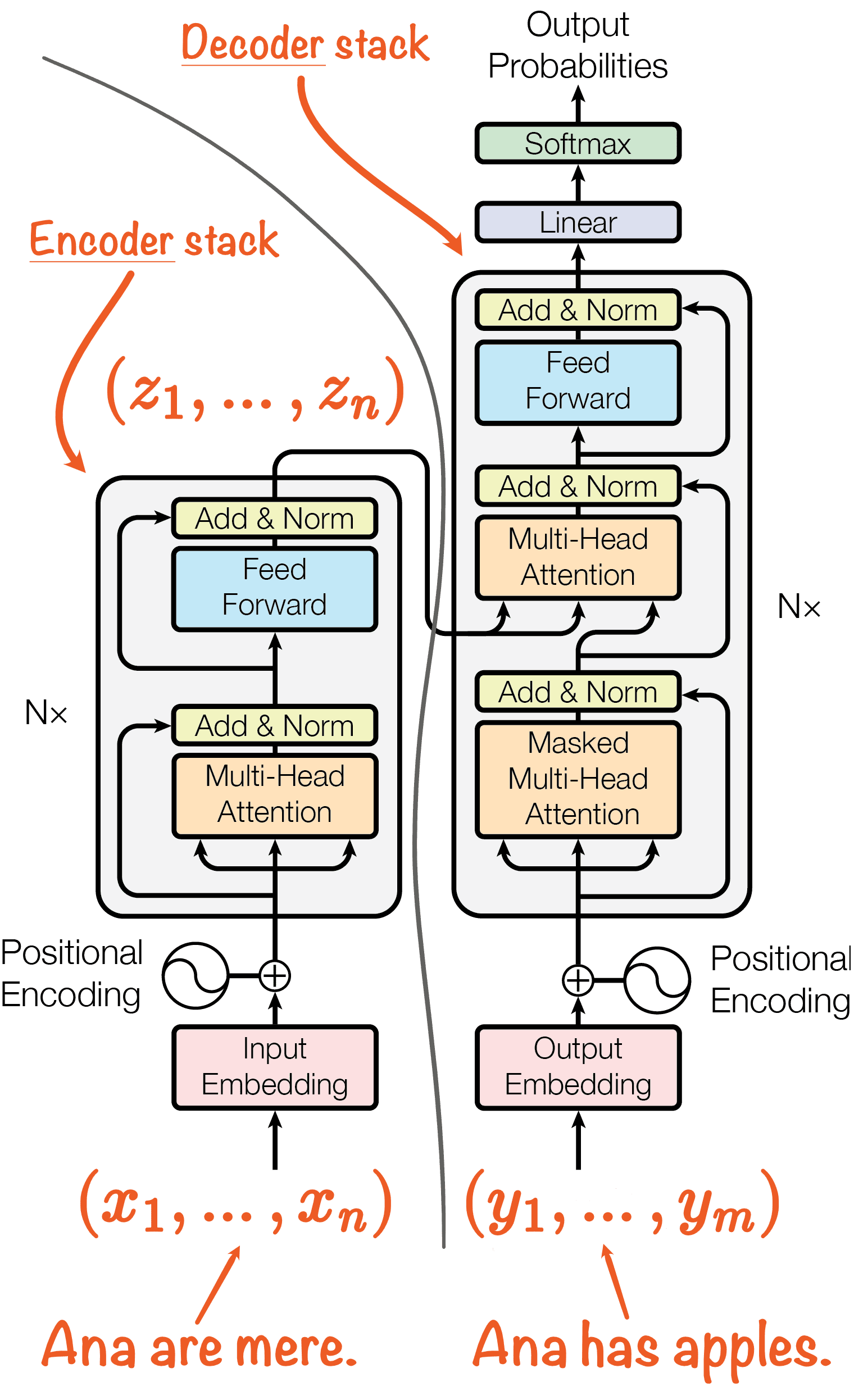
The encoder maps an input sequence of symbol representations
(x1,…,xn) to a sequence of continuous representations
z=(z1,…,zn). Given z, the decoder then
generates an output sequence (y1,…,ym) of symbols one element
at a time. At each step the model is auto-regressive, consuming the previously
generated symbols as additional input when generating the next.
Encoder and decoder, huh? In plain language, as part of this transformation,
the Romanian input is encoded by the model into an internal
representation, which is then decoded into English, one word at a time.
Let’s put this on the diagram. You can see the two halves: where the input goes
in, what produces the internal representation, and where the output comes out.
The z=(z1,…,zn) at the top of the encoder is that
internal representation, often called the latent (hidden) representation.
There are no words there, only a list of vectors that capture the phrase’s
meaning rather than its spelling.
The annotations look backward: Output arrows go into the Transformer
but somehow that’s considered the output? We’ll solve that after a short
detour.
GPT
In the intro, I drew a timeline from the Transformer to ChatGPT-like LLMs.
Before it becomes confusing, I need to draw a line from machine translation
models to chat and agentic models.
In chat and agentic models, we don’t want our input to be transformed. We want
the model to respond to it. To make this happen, we figured we could ignore the
encoder side, pass the input as if the decoder wrote it, and let it continue
it. We take that newly written output as the model response.
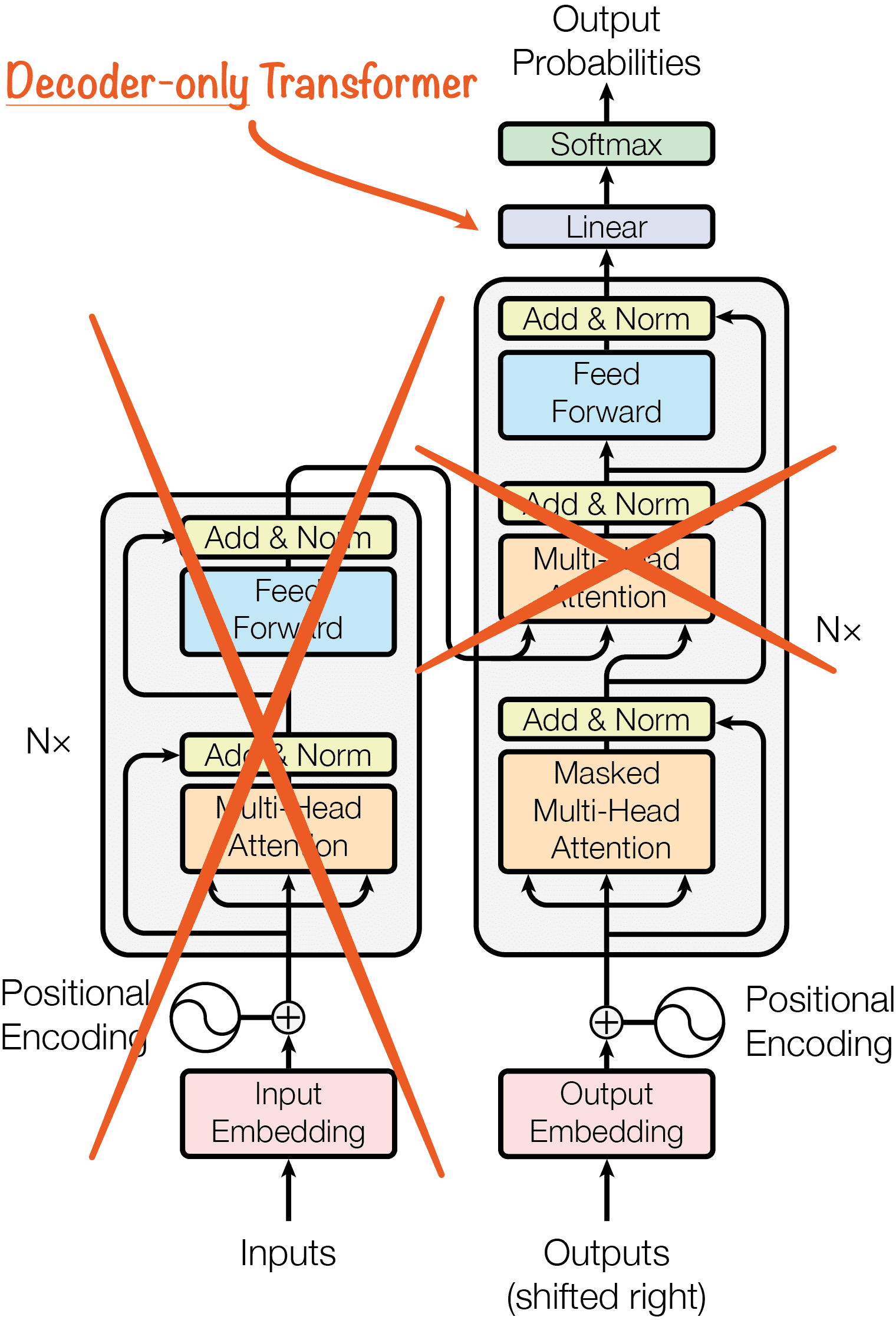
The original ChatGPT and pretty much all LLMs today are built only on the
decoder stack of the Transformer, the right side of the diagram above (minus the
middle attention block that connects the encoder). Such models are called
decoder-only Transformers. The decoder is the half that generates, which
gives us the G and the T in GPT.
There’s more though, encoder-only Transformer variants also exist and are
actively used for tasks such as classification, semantic similarity, etc. It is
impressive how many problems have been influenced by this paper. We are getting
a taste of why it is such a big deal.
Auto-regressive Generation
Why do Output arrows go into the Transformer? It makes more sense if we
rewind the translation a couple of steps:
Remember the last sentence of the opening paragraph of the Model Architecture section:
At each step the model is auto-regressive, consuming the previously generated
symbols as additional input when generating the next.
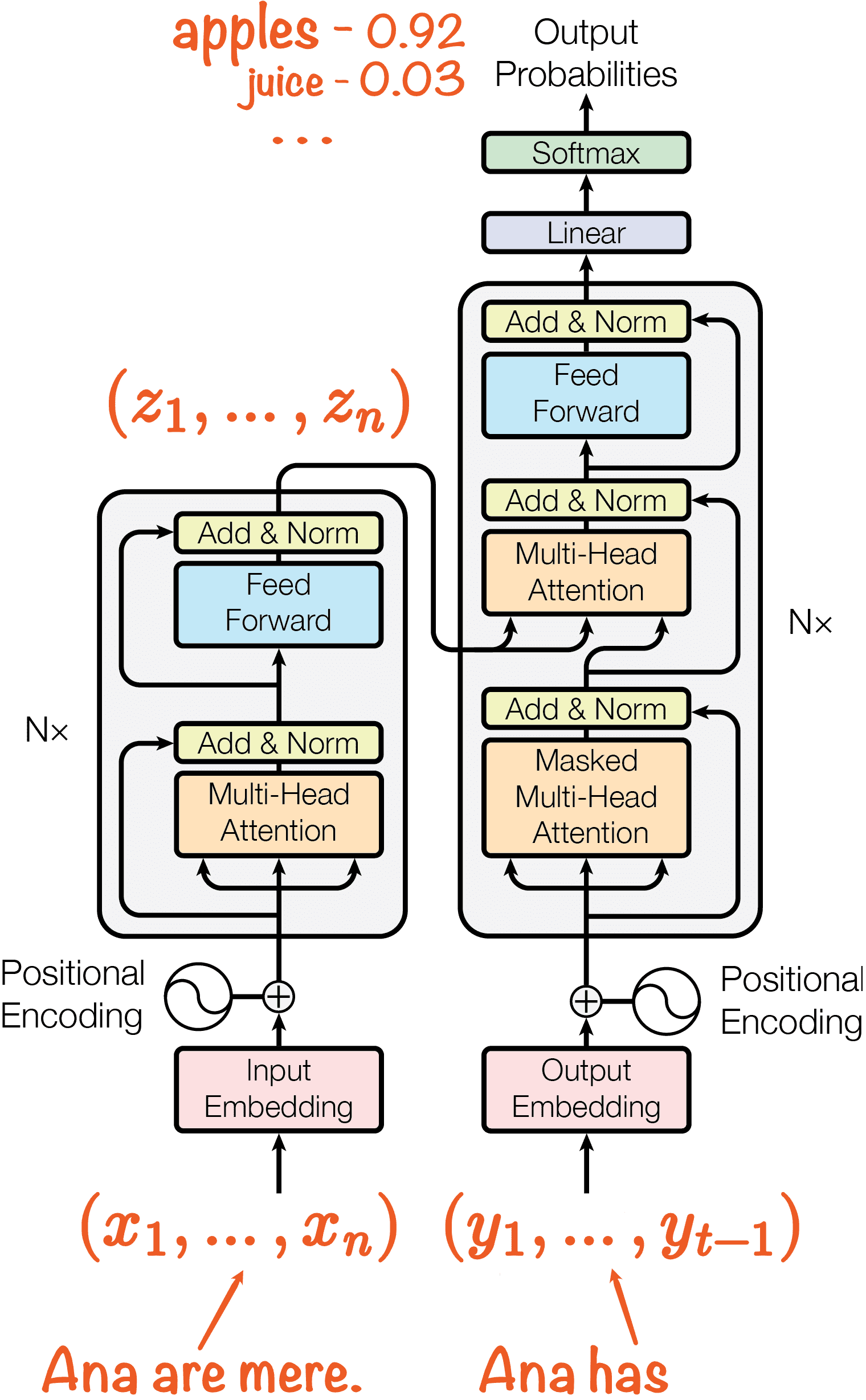
So before the word apples is predicted, we pass the previously generated output Ana has
into the model and the model predicts the next word. In this case apples by giving it
a probability of 0.92.
There are three missing details from the diagram to make it complete at this
level of abstraction. One of them is probably already on your mind: How do we know
when to stop generating new words? For this, we use a special word: EOS (End of
Sequence). When the model picks it as the next word, we stop.
The second is that the decoder doesn’t output just one probability distribution
for the next word. It outputs one for every position in the
output sequence y, predicting the word that follows that
position.
This creates a chicken-and-egg problem: if every word is predicted from the
position before it, where does the first word come from? To solve this, we
introduce another special word, the third missing detail:
BOS (Beginning of Sequence) and put it in the first position.
The distribution at that position gives us the first word.
At this conceptual level, the complete diagram of the last step looks like this:
Each term P(yi∣y<i,x) at the top is the probability distribution,
over every single word the model knows, for position i, given the output words
before it, y<i=(y0,…,yi−1), and the whole Romanian phrase x.
From Text to Numbers
Now that we understand what happens outside the Transformer, let’s start the
journey of understanding what’s happening inside. We start with our original
phrase, Ana are mere., and see how it makes its way into the encoder
(reminder: the left side of the Transformer).
"Ana are mere."?(x1,…,xn)
I’ve deliberately avoided an exact mapping from the phrase’s words onto x and y
above, the reason being that they don’t map directly: these models don’t
really operate on words. They operate on … tokens. Bingo!
Imagine for a moment that the model operated on words, and think about what the
output looks like: a probability distribution over every single word the model
knows. How many words are in the English language? In all known languages?
Now add misspellings, invented words, numbers, etc. And no matter how long we
make the list, someone will type a word that isn’t there. Just thinking about
this causes a headache, and it only gets worse as we look inside the model.
The trick is to find something that can be used to build all possible
words. But it can’t be too small, or that causes other issues.
That is the tokenization problem.
Here, I won’t get into its details and will use GPT-2’s tokenizer,
r50k_base. It’s based on byte-pair encoding (BPE), similar to what the
paper used for English-German translation.
r50k_base has a list of 50257 tokens, its vocabulary. The position of a
token in this list is its token ID. These IDs are what the x and
y sequences are made of.
"Ana are mere."↓⏐tokenize(An,a,␣are,␣mere,.)↓⏐as IDsx=(x12025,x264,x3389,x45019,x513)From text to tokens in Python (click to open)
# tokens.pyimport tiktoken
enc = tiktoken.get_encoding("r50k_base")
text ="Ana are mere."
ids = enc.encode(text)
tokens =[enc.decode_single_token_bytes(i).decode(errors="replace")for i in ids]print(f"{text!r}: {tokens} -> {ids}")
For the output, we will go the other way: pick a token ID from each probability
distribution, then turn the IDs back into text.
Note: r50k_base has no separate ⟨BOS⟩ and
⟨EOS⟩ tokens. One special token,
<|endoftext|>, plays both roles.
Through the Encoder
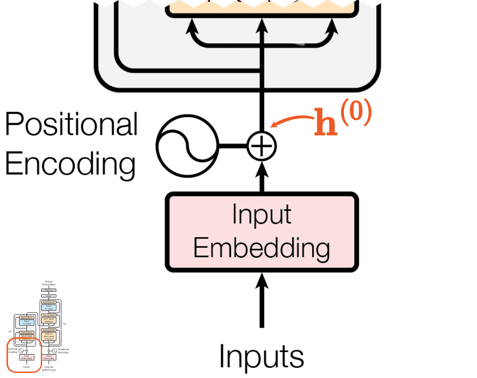
Each token ID is associated with a vector. In the paper, the size of these
vectors is dmodel=512 (Sections 3.1 and 3.4). Stacked together, they
form the embedding matrix E∈R50257×512, one row per
token ID. In the diagram, this matrix is the Input Embedding box. This is the
first time we meet some of the model parameters—numbers the model learns.
The box next to it, Positional Encoding, is a list of vectors too, this time
one per position; we’ll call this matrix PE. Unlike the embeddings, they are
computed from the token positions rather than learned. These vectors are what
let the encoder distinguish between two different arrangements of the same
tokens. That’s all we need for the purpose of this note; see Section 3.5
Positional Encoding of the paper for details.
Back to our example, Ana are mere.: for each token, we look up its learned
embedding (its row of E), add the positional encoding for its position (a row
of PE), and get the encoder input, our first hidden state z(0):
Note: positions count from 0, as in the paper’s code, so the first token x1
gets PE0.
The result z(0) is a table of numbers with one row per token and
512 numbers per row. Numbers are made up.
z(0)=0.120.571.35−0.47−0.710.521.19−0.34−1.340.070.910.680.210.52−1.05⋯z1(0)⋯z1(0)⋯z1(0)⋯z1(0)⋯z1(0)1.330.481.191.880.79512 numbers per row←z1(0)←z2(0)←z3(0)←z4(0)←z5(0)Ana␣are␣mere.
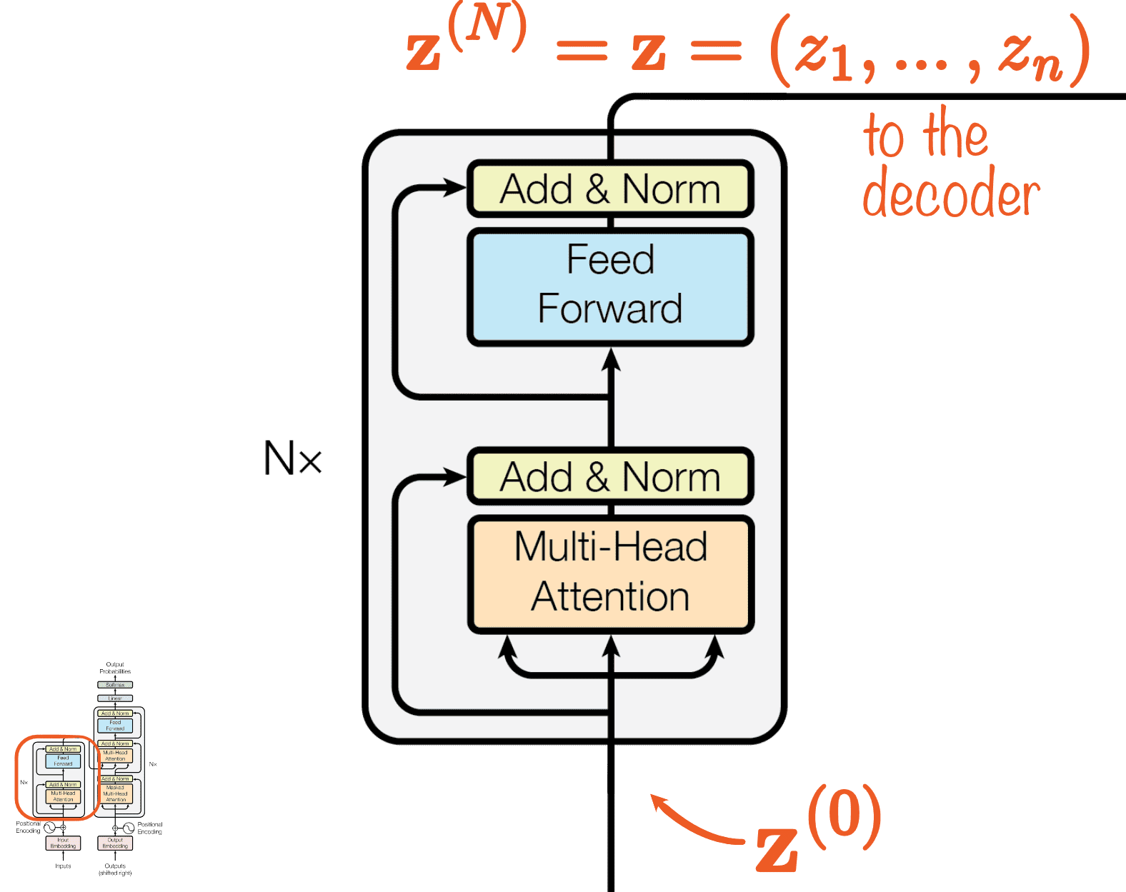
This hidden state makes its way into the encoder stack, which in the paper has
N=6 layers.
We’ll denote the output of each layer z(1),…,z(N).
The output of the last layer is what we referred to as the latent
representation, written without a superscript: z=z(6).
Note: capital N is the number of layers (6), while lowercase n is the number
of tokens (5 for Ana are mere.). The two are unrelated.
All these outputs have the same size, 5×512. Remember, Ana are mere.
has 5 tokens. The 512 is a design choice, a hyperparameter that worked
well for the problem at hand.
z(ℓ)=EncoderLayer(z(ℓ−1);θℓ),ℓ=1,…,N
Every layer runs the same computation, EncoderLayer, with its own
parameters θℓ. That makes two kinds of model parameters so far: E
and the θℓ.
Inside an Encoder Layer
Let’s unwrap EncoderLayer and figure out why there is a 🔱 trident. I still
need to squint quite a bit to understand the intention, so don’t worry if it
looks confusing at first.
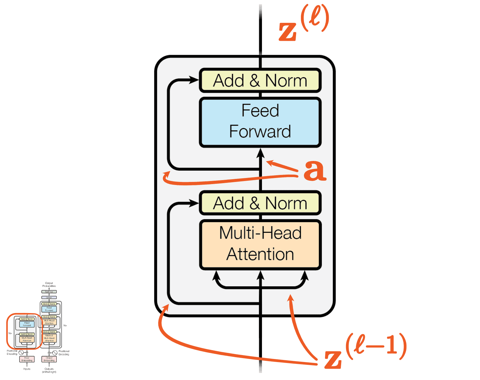
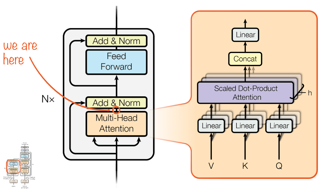
The layer input, z(ℓ−1), goes through Multi-Head Attention
first. We add the attention output back to the input, a residual connection,
and normalize the sum (Add & Norm). Normalizing rescales each token’s
numbers into the same range, so they don’t grow as every layer adds to them.
We’ll name the normalized sum a.
Then a goes through a feed-forward network, the Feed Forward box.
We add its output to a and normalize again.
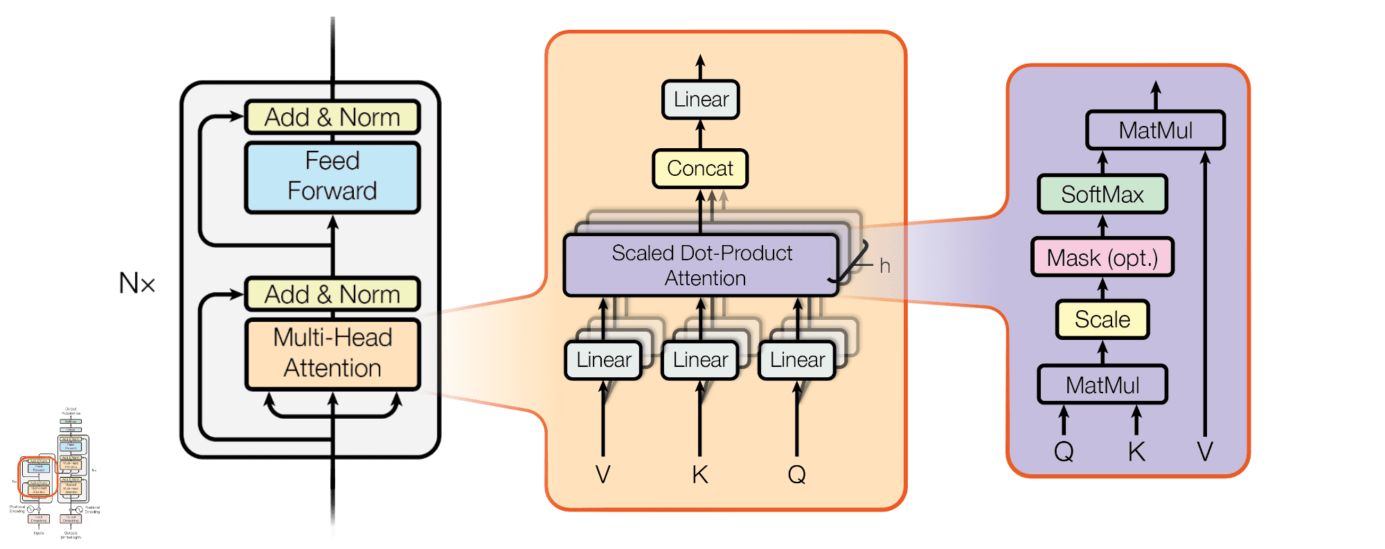
Let’s bring in two more diagrams from Figure 2 of the paper: Multi-Head
Attention and Scaled Dot-Product Attention.
Read the V (values), K (keys), and Q (queries) labels in the middle and right
sub-figures as names rather than objects. In code, they’d be function
parameter names. They might or might not correspond to the same value. In the
case of the encoder, all three inputs of the middle sub-figure carry the same
matrix: z(ℓ−1)! This is the trident we
saw earlier—binding the input to parameter names.
You can see that each of the V, K, Q lines on the diagram forks further into h
separate branches, the heads, matching its Multi-Head name. Think of each
head as an independent computation process. Each has the same structure and
its own parameters, so each can focus on different features of the input.
In the paper, the authors use h=8 heads. So the layer input
z(ℓ−1) inside Multi-Head Attention is really referenced
3×8=24 times: V, K, Q once for each head.
Inside an Encoder Attention Head
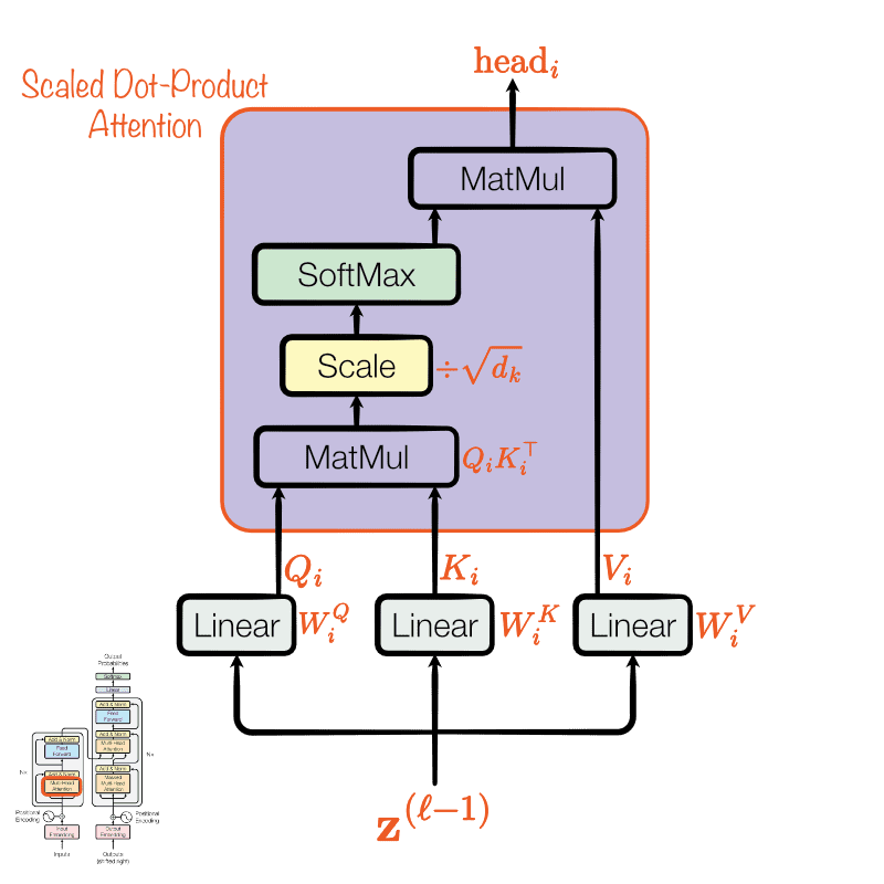
Let’s bring our attention (pun!) to a single attention head. I’ll zoom in
on the diagram and make it more concrete. For this one, I dropped the paper’s
Mask (opt.) box between Scale and SoftMax because only the decoder uses it;
we’ll get to it there.
Let’s follow the numbers first by looking at the queries
Qi=z(ℓ−1)WiQ.
We haven’t seen WiQ before. It is a matrix of learned parameters. Each row
of z(ℓ−1) carries information about one token. Multiplying the
two projects the input sequence into a list of questions. Keep this abstract
for now.
Let’s look at the keys Ki=z(ℓ−1)WiK.
As with the queries, we project the input sequence into a list of keys.
If you follow the row-by-column matrix multiplication, you’ll notice that there
is no interaction between the elements of the input sequence! In the first
layer, the only signal comes from the token itself and its position in the
input sequence.
This brings us to the first operation of Scaled Dot-Product Attention:
QiKi⊤:
The result is a 5×5 matrix of attention scores: row t says how
much attention position t pays to every position in the input sequence,
itself included. Every entry is a dot product, which measures how well
a query and a key line up.
Each score adds up 64 products (the size of each query and key,
dk=dmodel/h=512/8), so the scores get large. Scale
divides them by dk=8, and SoftMax makes them relative by
turning each row into a split of attention that sums to 1:
softmax(x)s=∑rexrexs
For the ␣are row, with made-up scores:
An
a
␣are
␣mere
.
raw score
3
−6
9
22
−4
÷ 8
0.375
−0.75
1.125
2.75
−0.5
SoftMax
0.068
0.022
0.145
0.736
0.029
␣are puts 74% of its attention on ␣mere and 14% on itself. Without Scale,
␣mere would take 99.9998%. The authors suspect such extremes make training
hard (Section 3.2.1).
The result is a 5×5 matrix of attention weights, one row per token:
softmax(dkQiKi⊤)
Let’s look at the values Vi=z(ℓ−1)WiV.
As with the queries and keys, we project the input sequence, this time into
a list of values: the information each token passes on when another token
attends to it.
Remember the trident? Queries, keys, and values all come from the same
z(ℓ−1): the sentence is attending to itself. That’s the self
in self-attention.
Now that we’ve figured out the attention between the tokens, let’s make the
information actually flow. So far, nothing has moved: the weights only say who
listens to whom. The last MatMul does the moving. Let’s call the weights
α:
Each row of α is one token’s split of attention, and each row of Vi
is one token’s value. Multiply them, and row t of headi becomes a
blend of all the values, mixed in the proportions of αt. Here’s the
blend for ␣are, with the weights from the table above:
␣are comes out 74% ␣mere’s value, 14% its own, and the rest from the other
tokens. Every row gets its own blend.
Before this MatMul, each row of Vi came from one row of the input. Now each
row of headi carries something from the whole sentence.
In the first layer, an input row knows only its own token and position. From
the second layer on, it already carries context from the layer below, so each
layer builds on the ones before.
That’s one head. The other seven do the same with their own weights, and each
produces its own 5×64headi.
Putting the Heads Together
Back to the Multi-Head Attention diagram. Two boxes are left above the heads,
Concat and Linear. Together they compute:
MultiHead(Q,K,V)=Concat(head1,…,headh)WO
Concat puts the eight heads side by side. Each token’s row grows from 64 to
8×64=512 numbers, back to dmodel:
Each color is one head’s 64 columns. Row ␣are now holds eight blends of the
sentence, one from each head. The heads haven’t seen each other’s results yet.
Linear multiplies by one more matrix of learned parameters,
WO∈R512×512:
Each output number is a row of Concat times a column of WO, so it mixes all
eight heads. Attention mixed information across tokens, the rows. Linear mixes
across heads.
So far, we’ve mostly mixed information between tokens with fairly
simple linear projections (all those Linear boxes we saw). The Feed
Forward box takes it to the next level: this is where much of the interesting
computation happens.
The feed-forward network is one of the oldest building blocks of SI:
a multilayer perceptron (MLP) with one hidden layer (Section 3.3).
One interesting detail about this computation: it runs on each token
independently. I’ll hand-wave here and say that we’re computing something
about each token.
And the final residual connection and norm, same as the
first one:
z(ℓ)=LayerNorm2(a+FFN(a))
Six Layers Later
That’s one encoder layer. The stack repeats it N=6 times, each time with
its own parameters θℓ:
z(0)θ1z(1)θ2⋯θ6z(6)=z=(z1,…,z5)
Out of the last layer comes z, the latent representation from the
overview: a list of vectors that capture the phrase’s meaning rather than its
spelling.
Encoder-Only Models
This was the encoder: halfway through the Transformer, but an important
milestone. Remember I mentioned encoder-only variants? If you’ve heard
about classification or similarity problems, that’s pretty much what’s behind
them. Their outputs are built on this meaningful representation.
Google’s BERT (2018) is the best-known encoder-only model. Its output is
z, and we put it to work with a small extra step on top.
TODO: Explain the BERT name (Bidirectional Encoder Representations from
Transformers). Good spot to point out that the encoder’s attention is
bidirectional: every token sees every other token, both before and after it.
Set up the contrast with the decoder, which comes next.
For classification, a small classifier turns z into a label:
positive or negative, spam or ham, which topic.
For similarity, we pool z into one vector, for example by
averaging z1,…,z5. In models built for this, phrases with similar
meaning get vectors that point the same way, and cosine similarity (a dot
product of the vectors scaled to length 1) tells us how well they line up, just
like queries and keys, minus the length. This is what powers semantic search.
Through the Decoder
But the main reason we’re here is to turn this meaningful representation back into text, English text.